-
 fdrake
7.2kSo I think §2 is reasonably straight forward, it's an exercise of the imagination which sets out what Riemann means when he thinks of a multiply extended magnitude.
fdrake
7.2kSo I think §2 is reasonably straight forward, it's an exercise of the imagination which sets out what Riemann means when he thinks of a multiply extended magnitude.
§ 2. If in the case of a notion whose specialisations form a continuous manifoldness, one passes from a certain specialisation in a definite way to another, the specialisations passed over form a simply extended manifoldness, whose true character is that in it a continuous progress from a point is possible only on two sides, forwards or backwards.
I think the archetypal example here is that of a line segment. I think a specialisation can be harmlessly read as a dimension, or direction of variation. So say we have the following line segment:
(-------)
the specialisations we pass over are the points which constitute it, and together they form the line - the simply extended manifoldness. There are only two directions to travel, forwards and backwards, and this gives the 'true character' of it. This notion is, however, broader than a line, as the boundary of a circle would also be a simply extended manifoldness: we are only travelling 'forwards' through clockwise rotations and 'backwards' through anticlockwise rotations, assuming we lay on the circle's boundary.
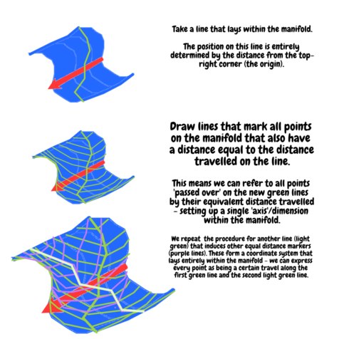
Inherent in this is the idea of parametrising a movement with respect to the changes in a single direction of variation, and one common way of doing this is by parametrising the position on a shape by the distance required to travel to it while remaining within the shape, the arclength.
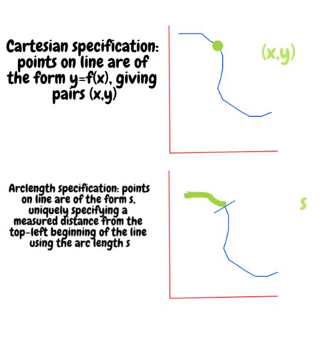
Thinking about it in terms of travel on the manifold (the line above) reveals how many directions of variation are required to express its variations innately - we only need one, the arc length, because it's one dimensional. This is a simply extended manifoldness, one of a single dimension.
If one now supposes that this manifoldness in its turn passes over into another entirely different, and again in a definite way, namely so that each point passes over into a definite point of the other, then all the specialisations so obtained form a doubly extended manifoldness.
Now we make the above blue line 'pass over' another red line, creating a doubly extended manifoldness:
which, note, can have the points on it described by the arclength along the first blue line and the arclength along the second red one (the arrow). This means it is 2 dimensional (despite it being embedded in 3-space).
In a similar manner one obtains a triply extended manifoldness, if one imagines a doubly extended one passing over in a definite way to another entirely different; and it is easy to see how this construction may be continued. If one regards the variable object instead of the determinable notion of it, this construction may be described as a composition of a variability of n + 1 dimensions out of a variability of n dimensions and a variability of one dimension.
And Riemann iterates the procedure, giving a recipe for constructing a manifold of n+1 dimensions from a manifold with n dimensions and a manifold of 1 dimension. This procedure is usually called 'sweeping out' space, and usually first appears in undergraduate or school calculus when discussing volumes of revolution, the Wiki link there has another good picture of 'sweeping out' a 2 dimensional surface using a 1 dimensional surface (and a circle/axis of rotation).
Another thing to highlight here is that Riemann is looking at composing higher dimensional shapes out of lower dimensional shapes; the dependence on the coordinate system used to express either is like map to the territory, the shapes are the shapes, the manifolds are the manifolds, regardless of the particular coordinate system used in their description. -
 Streetlight
9.1kHard to add to what @fdrake already laid out for §2, so maybe just a bit of 'how Streetlight intuits it' kind of thing. So, my approach has been to think of an 'extended magnitude' as something like a 'shaped dimension' - a dimension with a shape. In fact, we can begin with dimensions and use them to think n-ply extended magnitudes. So here's a nice image I found illustrating dimensions:
Streetlight
9.1kHard to add to what @fdrake already laid out for §2, so maybe just a bit of 'how Streetlight intuits it' kind of thing. So, my approach has been to think of an 'extended magnitude' as something like a 'shaped dimension' - a dimension with a shape. In fact, we can begin with dimensions and use them to think n-ply extended magnitudes. So here's a nice image I found illustrating dimensions:
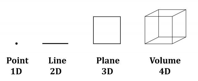
This kind of thing should be relatively familiar with most people. Now, ignoring the 1D point (which doesn't have a magnitude or size), a 1D extended magnitude actually corresponds to the 2D line: the line is the most basic 'extended magnitude' along which one can move backward and forward along. Now, add another dimension (the 3D plane) and you have a doubly (2-ply) extended magnitude. Add yet another, and you have a triply (3-ply) extended magnitude and so on, for all dimensions N - hence, n-ply extended magnitudes. 'Adding dimensions' is what Riemann refers to as a manifold 'passing over into another entirely different manifold in a definite way'.
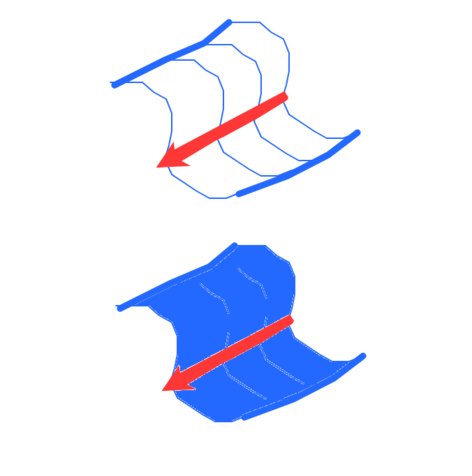
The only thing to add to this is that extended magnitues, unlike the 'dimensions' we're used to speaking about (pictured above) don't have to be straight. They can be bendy. Or to use a more technical vocabulary, they don't have to be rectilinear, they can be curvilinear, like fdrake's illustrations. So if you begin with a bendy 1D extended magnitude (a curvy line), you can 'pass over' into another magnitude by rotating the curve. From the fdrake's Wiki link:

This is a 1-ply extended magnitude (a bendy 2D line) 'passing over' into a 3-ply extended magnitude (a 4D Volume). This 'skips' the 2-ply extended magnitude because we're rotating the curve, rather than just 'stretching it out' along a single dimension, like was done in fdrake's post. -
Streetlight
9.1kOne thing that I've taken for granted in the above presentation is the fact that dimensions are always 'one number higher' than n-ply extended magnitudes. So a 2D line corresponds to a 1-ply extended magnitude, a 3D plane corresponds to a 2-ply extended magnitude and so on. Again, as fdrake points out, this difference is vital. In a Cartesian coordinate system, a point is specified by as many variables as there are dimensions. I.e:
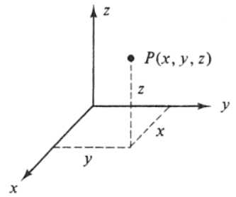
Point P is specified by 3 variables, x, y, and z, corresponding to each of the spatial dimensions of the coordinate system. If, however, point P were to be part of a 2-ply extended manifold (which, remember, corresponds to a 3D plane), one would only need 2 variables, and not 3. And the reason this is so, is that the measure of the magnitude is no longer extrinsic to the surface (like the Cartesian coordinates), but immanent to it. This also has to do with why the measure of magnitude starts with a curve (a line is species of a curve, btw), and not a point. Only a curve can have a magnitude, which is why n-ply magnitudes are always one number 'down' from a dimension. -
fdrake
7.2k
Quick corrective note: Riemann equates simply extended magnitudes with 1 dimensional objects, but the points which constitute them are 0 dimensional. So the point/line/surface/volume are 0/1/2/3 dimensional respectively. In my diagrams, we have a curve passing over another curve, and because it's 2 curves passed over we have 2 dimensions.
He switches to the dimension vocabulary in §3
I shall show how conversely one may resolve a variability whose region is given into a variability of one dimension and a variability of fewer dimensions. To this end let us suppose a variable piece of a manifoldness of one dimension - reckoned from a fixed origin, that the values of it may be comparable with one another - which has for every point of the given manifoldness a definite value, varying continuously with the point...
this procedure, taking a variability of one dimension (a curve) from a manifoldness of higher dimension n, reduces the remaining dimensions of the manifold left unaccounted for by 1. So we end up with n-1 directions for variation when we've already set up the 'variability of one dimension' - a 'simply extended magnitude', since it 'varies continuously with the point'. -
fdrake
7.2kThis is a 1-ply extended magnitude (a bendy 2D line) 'passing over' into a 3-ply extended magnitude (a 4D Volume). This 'skips' the 2-ply extended magnitude because we're rotating the curve, rather than just 'stretching it out' along a single dimension, like was done in fdrake's post. — StreetlightX
If you want to consider the volume of the vase, then the whole circle is a 2 dimensional object we're 'passing over' with the curve which is a cross section of the vase boundary, adding the dimensions gives us that the resultant manifoldness would be of 3 dimensions. If instead we rotate the curve which is a cross section vase boundary solely along the boundary of the circle (the full extent of the radius), we end up with a 2 dimensional vase-surface, since the circle boundary is 1 dimensional and the vase boundary is too (which is what's actually pictured in the wiki link, but it is using this procedure to suggest the volume itself is formed from the rotation by setting up the right vase-boundary). -
fdrake
7.2kRiemann has given us a method for constructing higher dimensional manifolds from lower dimensional manifolds. In §3 he does the reverse, giving us a method to decompose higher dimensional manifolds into lower ones. He switches to the vocabulary of dimensions/variations in the first paragraph of §3, and we can consider each dimension as devoted to a simply extended manifoldness:
I shall show how conversely one may resolve a variability (manifoldness-me) whose region is given into a variability of one dimension and a variability of fewer dimensions. To this end let us suppose a variable piece of a manifoldness of one dimension (simply-extended, me) - reckoned from a fixed origin, that the values of it may be comparable with one another - which has for every point of the given manifoldness a definite value, varying continuously with the point; or, in other words, let us take a continuous function of position within the given manifoldness, which, moreover, is not constant throughout any part of that manifoldness.
'not constant' is a requirement for being a coordinate axis, say if on the usual real line every number between 0 and 1 was normal, it was associated with the correct real number, but every number above 1 was associated with the number 2. This would mean that this direction of variation cannot discriminate between positions which must be represented as quantities greater than 2, 'folding' all of the real line between 2 and infinity into the natural number 2. Riemann describes the procedure as something that looks like this:
(click to zoom) We also could have used distance along the original blue line and the original red arrow as axes, but I wanted to stress that any other pair of independent directions of variation within the manifold would do the same job. This procedure usually works, so long as the dimension of the manifold is finite and that the coordinate system doesn't have singular points. Riemann stresses that infinite dimensional manifolds do exist and are worthy of study:
There are manifoldnesses in which the determination of position requires not a finite number, but either an endless series or a continuous manifoldness of determinations of quantity. Such manifoldnesses are, for example, the possible determinations of a function for a given region, the possible shapes of a solid figure, &c
such as manifolds whose points consist of functions (function spaces) or shapes. This concludes 3 - Riemann's discussion is just describing the above picture and its limitations. -
fdrake
7.2kHere's another demonstration of 'innate coordinates', using the simply extended manifoldnesses (1D manifolds) of the original blue curve and the red arrow to express the position of a point on the doubly extended manifoldness formed from 'sweeping one over the other'.

The black point is what you get when you travel the green point along the blue curve and the lilac point along the red curve. This is equivalent to the usual notion that the coordinate (1,2) in the x-y plane is obtained by going forward along the x/horizontal axis by 1 and forward up the y/vertical axis by 2. Only now we're moving over curves rather than straight lines - transitioning from rectilinear to curvilinear coordinates as @StreetlightX highlighted here. -
fdrake
7.2kAnother thing which is worthwhile to highlight is that coordinate systems are a way of ascribing positions based on quantities - so we have length magnitudes characteristic of position being translated to numbers which measure the lengths in some system of measurement (coordinate system).
Riemann follows this connection between measurement/metric and coordinate system in the next section. -
 Moliere
6.5kA point of clarification for me. I'm trying to wrap my head around the idea that you only need one number to specify your location on a 2-dimensional line.
Moliere
6.5kA point of clarification for me. I'm trying to wrap my head around the idea that you only need one number to specify your location on a 2-dimensional line.
The only way I can think that this is possible is if, on every point of the line there is a unique value for that line -- so that you really do only need 1 number to specify your location, the arclength (or whatever), since your position cannot be any other position due to every position being unique.
But otherwise I'm not tracking. -
fdrake
7.2kA point of clarification for me. I'm trying to wrap my head around the idea that you only need one number to specify your location on a 2-dimensional line. — Moliere
Switching into the language of degrees of freedom can help. A degree of freedom is a unique direction of variation. Straight lines have 1 degree of freedom. If you remember from school straight lines have the equation:
this means if you fix , you determine immediately. The same concept holds for, say, the boundary of a circle. The points laying on the boundary of a circle (with radius 1 centred at the origin) satisfy the equation:
this means that if you fix an , you can determine the (up to sign). Another way of seeing this dependence on a single variable is that you can uniquely specify a point on the boundary of a circle through an angle of rotation:
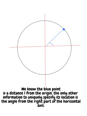
So when the usual degrees of freedom for expressing a position in space using an angle and a distance from the origin are... the angle and the distance from the origin... and if we constrain the distance to be constant (1, here), we lose a degree of freedom (dimension) from the unconstrained space (of 2 dimensions) by applying one constraint (the distance from the origin = 1).
When I showed this with my examples of a 2 D shape with lines on it above, each line creates axes across the shape where the distance would be the same. In the second diagram in that post. I've added the 'lines of constant distance' from the original blue curve we used to sweep over the red one, pictured below.
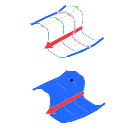
The green curve denote all the possible positions consistent with being the picked distance travelled on the blue curve, the lilac curve denotes all possible positions consistent with being the picked distance travelled on the red curve. You can see they intersect at one and only one point, the previously specified black one - this is why the black one showed up in the place that it it did. -
Moliere
6.5kAlright, I think I'm tracking now. I wasn't thinking of the line as somehow "fixing" position, and was caught up on thinking about how I'd actually find my position on the line -- sort of thinking about it like it is in a Cartesian coordinate: I know both yourself and @StreetlightX basically said to not do that, but them's where I was.
But the line example is more general than that -- it's not a function, per se, it's just a representation of a manifold which happens to have that shape. So if a manifold were shaped like a sphere, for example, and that sphere is already "given" in the sense that we already know how far each point is from the origin (if we so chose to express it in such and such a coordinate system), then we would only need 2 numbers to find our position on said sphere.
If this sounds right, then I'd say your circle example helped a lot -- I wasn't thinking of it as having already been "fixed" and was stuck on trying to figure out how I'd find where I was on a coordinate system. -
Streetlight
9.1kOkay, I think I know where I got confused: in my attempt to distinguish between dimensions and n-ply magnitudes, I conflated certain things. For instance, rectiliear and curviliear lines: rectilinear lines are 1D, and curvilienar lines are 2D, but as far as treating them as manifolds is concerned, there is no real difference. So this doesn't map neatly on my attempt to simply specify that n-ply variables are always one degree 'down' from a dimension. I made a similar conflation between extended S-curves and the vase - I thought the vase would be a +1 degree manifold over a S-curve, but I was wrong about that. So. Here's a diagram I drew:
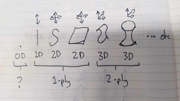
Does this look right?
I'm still confused about the OD point: does it count as an extended magnitude or not? -
fdrake
7.2k
That sounds about right Moliere. You extended it correctly (by my reckoning) to the surface of the sphere, so I think we see eye to eye now.
I'm still confused about the OD point: does it count as an extended magnitude or not? — StreetlightX
Typically it doesn't, and I don't think it does for Riemann either. From the §1 in section one:
Magnitude-notions are only possible where there is an antecedent general notion which admits of different specialisations. According as there exists among these specialisations a continuous path from one to another or not, they form a continuous or discrete manifoldness; the individual specialisations are called in the first case points, in the second case elements, of the manifoldness
The important line is:
According as there exists among these specialisations a continuous path from one to another or not, they form a continuous or discrete manifoldness; the individual specialisations are called in the first case points
removing the parts which aren't talking about 'continuous manifoldness' or 'points' and paraphrasing:
According as there exists among these specialisations a continuous path from one to another or not, they form a continuous manifoldness (whose specialisations consist of) points
we have that 'points' are a specialisation of which 'manifoldnesses' consist of just when 'there is a continuous path between (every pair of) points'. Now that we've established that specialisations are points, and continuous manifoldnesses consist of points, Riemann develops the notion of a continuous manifoldness in §2:
If in the case of a notion whose specialisations form a continuous manifoldness, one passes from a certain specialisation (point 1) in a definite way to another (point 2), the specialisations passed over form a simply extended manifoldness (a path between points - a line or curve), whose true character is that in it a continuous progress from a point is possible only on two sides, forwards or backwards (in the direction of increasing or decreasing arclength).
So we have that simply extended continuous manifoldnesses consist of points. Simply extended manifoldnesses are 1D objects, because 'in it a continuous progress is possible only on two sides' - like the horizontal axis in Cartesian coordinates; we can go right or left, and going right is the same as going 'inverse' left, like up and down are both part of the vertical dimensions, left and right are both part of the horizontal dimension, 'forward and backward' denote the union of the two directions within a single axis.
In answer then, an isolated point is not a 'simply extended manifoldness', or a 1 dimensional object, because for it no 'progress' is possible. Thinking intrinsically, if you placed your point of view on the point, there are no possible movements you can make in any direction to still remain on the point - you have no degrees of freedom for motion - since your position is completely specified. This total lack of degrees of freedom; corresponding to the complete specification of a location; is why a point is 0 dimensional.
Though Riemann has not ascribed a dimension to points in the paper, only to manifoldnesses which consist of points (in the continuous case). The lowest dimension being a simply extended manifoldness or 1-ply extended magnitude (a line or curve with infinitesimal/0 thickness, strictly speaking I think n-ply magnitudes are associated with n dimensional manifoldnesses, rather than being equivalent to them, but this equivocation here helps more than it hinders. I think later n-ply extended magnitude is a coordinate system notion, which can be used to describe positions on an n dimensional manifoldness). -
fdrake
7.2kMade a thing with more examples.
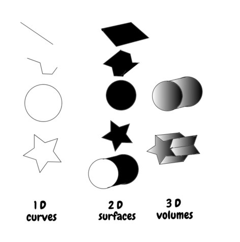
Empty areas in the 1D case because we're just considering the lines. Black areas in the 2D case mean we're dealing with all those shaded points in the enclosed area. Graduated shading areas in the 3D case means we're dealing with all those shaded points in the enclosed volume. The surface of a sphere is another example of a 2D manifold. All the points in a cube and all the points in a sphere are more examples of 3D manifolds.
Edit: imagine yourself on the manifold, with all the directions of movement the manifold allows you. 1D manifolds - you can only step forward and backwards. 2D manifolds - you can step forward and backward; and left and right, like walking on the floor of your house. 3D manifolds - you can go forward and back, left and right, and up and down - aeroplanes move in 3D, so do swimmers. If you can 'immerse yourself' in the manifold, you're in 3 dimensions. If you can 'move about freely on a surface' you're in 2 dimensions. If your movement is forced to move along a pre-determined path, your only choice being to move forward or back, you're in 1 dimensions. If you have nowhere else to travel, and no directions to travel in, without leaving the manifold you're on - you're on a point.
EDITED: Later developments in math have that 1 dimensional manifolds become associated with lengths, 2 dimensional manifolds become associated with areas, 3 dimensional manifolds becomes associated with volumes (measure theory). However the paper develops notions of inter-point distances (metrics - distance measuring functions) that lay within manifolds, rather then just dealing with the embedding space (example will be drawn later). -
fdrake
7.2k
-
fdrake
7.2kI'm going to move onto section 2 tonight, but just the summary of section 1 and the preparatory remarks for the remainder of section 2. Hopefully this will serve to get us all on the same page before the gigantic and dense walls of text in the second section.
EDIT: references to areas and volumes that were here have been removed seeing as Riemann doesn't actually discuss them in the paper! He just talks about length notions within manifolds.
II. Measure-relations of which a manifoldness of n dimensions is capable on the assumption that lines have a length independent of position, and consequently that every line may be measured by every other.
The title itself is an orienting remark, the first section was:
I. Notion of an n-ply extended magnitude.
and now we've developed notions of n dimensional manifoldness (curves/surfaces/volumes), n-ply extended magnitudes (coordinate systems of 1/2/3 dimensions), we can link manifolds to measures of length through the following chain of associations:
n dimensional manifoldness -> n ply extended magnitude/n dimensional coordinate system -> measures of length
In moving from n-dimensional manifoldness to n-ply extended magnitude, we needed to be able to associate every point in the manifoldness with a collection of quantities in the n-ply extended magnitude, which takes the notion of the position of a point within/on a manifold and maps it to a corresponding quantity (or set of quantities) that locates the position of the point. This is the basic function of an n-ply extended magnitude or coordinate system.
Now that we have a machine which takes manifolds and labels all their points in a consistent manner, we can take the point labels and start to ask questions using them: what's the distance between a pair of points within/on the manifold and how is this related to the quantities we used to measure their position? IE, how can we link a coordinate system to a notion of length?
In §1 in section 1, Riemann stipulated that:
Measure consists in the superposition of the magnitudes to be compared; it therefore requires a means of using one magnitude as the standard for another.
we first superposed a number of independent directions of variation to describe the position of a point on/within a manifold - taking a point in it and mapping it to a coordinate like (x,y), now we're going to superpose all those independent directions of variation in order to ascribe a length to them, like sqrt(x^2+y^2) - mapping coordinates or relative positions to quantities that represent their size.
The mechanism that described the ascription of a coordinate system (n-ply extended magnitude) to a manifold looks like this:
for every point p on a manifold of dimension n, we have the unique ascription
where we have n numbers that uniquely and completely specify the position p within the manifold.
Setting up this conception was the topic of section 1, especially the passages on how to build a manifold of n+1 dimension out of a manifold of n dimensions and a manifold of 1 dimension (with its simply extended magnitude). Riemann summarises all of the previous developments in the paper as:
Having constructed the notion of a manifoldness of n dimensions, and found that its true character consists in the property that the determination of position in it may be reduced to n determinations of magnitude (breaking a sentence in two here)
Section 2 however introduces something more similar to the modern notion of the relationship between manifold and coordinate system. It looks very similar to the one developed in section 1, but we 'zoom in' to get a weaker condition - a more local description:
for every point p there exists some neighbourhood around it such that we have the unique ascription:
where we have n numbers that uniquely and completely specify the position p within the manifold.
And this manifold is locally flat when all the numbers are ascribed consistently with the usual Cartesian coordinates when we zoom far enough in- making the coordinate geometry look flat very close up. What we're going to do now is flesh out the second arrow in the flow chart:
n ply extended magnitude/n dimensional coordinate system -> measures of length
and Riemann summarises these intentions in the next part of the first paragraph:
... (Now) we come to the second of the problems proposed above, viz. the study of the measure-relations of which such a manifoldness is capable, and of the conditions which suffice to determine them.
He then provides preparatory remarks for the remainder of the study:
These measure-relations can only be studied in abstract notions of quantity, and their dependence on one another can only be represented by formulæ. On certain assumptions, however, they are decomposable into relations which, taken separately, are capable of geometric representation; and thus it becomes possible to express geometrically the calculated results. In this way, to come to solid ground, we cannot, it is true, avoid abstract considerations in our formulæ, but at least the results of calculation may subsequently be presented in a geometric form. The foundations of these two parts of the question are established in the celebrated memoir of Gauss, Disqusitiones generales circa superficies curvas.
Firstly,
These measure-relations can only be studied in abstract notions of quantity, and their dependence on one another can only be represented by formulæ.
connotes that we will be superposing the coordinates we have ascribed to points on the manifold in order to derive notions of distance using them. Mathematically this resembles taking every coordinate as part of a function that maps to a single number. Like we can take (x,y) and map it to sqrt(x^2+y^2) to get the distance of the point (x,y) from the origin. More formally, Riemann will be constructing a localised version of something like:
which takes every coordinate of a point, combines them in some way through algebraic (and differential) operations which produces a single quantity - which is a measurement of length. Riemann will make...
certain assumptions (which ensure that the length ascriptions) are capable of geometric representation; and thus it becomes possible to express geometrically the calculated results.
which correspond to this locally-flat condition - since the space we live in (at least in a present-at-hand sense @John Doe) looks to obey Euclidean geometry/be flat on small scales, we can only draw things which have this condition even if we can stipulate different notions.
Riemann gives a final head nod to Gauss before diving right into the characterisation of flat space - what is it that makes flat space flat? It will turn out to be a measure relation of the above form. -
fdrake
7.2kStarting §1 in section 2. It's very likely that I have some misconceptions and falsehoods in my presentation since it's outside of my comfort zone. So take what I say with a pinch of salt.
§ 1. Measure-determinations require that quantity should be independent of position, which may happen in various ways. The hypothesis which first presents itself, and which I shall here develop, is that according to which the length of lines is independent of their position, and consequently every line is measurable by means of every other.
Riemann is constraining his discussion to metrics, means of measuring distances in continuous manifoldnesses, which ascribe distances independent of the location on the manifoldness. Note that this is a way of assigning a notion of size to a notion of geometry, rather than measuring a specific shape. This notion is what sets up the meaning of length in a geometry, rather than an instance of measuring any particular distance within it. To be sure, objects (sub-manifoldnesses, neighbhourhoods etc) will have their sizes expressible through this notion of size, but the notion of size itself is a characteriser of the geometry rather than of any particular shape.
When you say the length of lines is independent of their position, what this means is that the distance notion applies the same everywhere in the space - there are no partitions acting on the size notion that create regions of distinct size ascriptions. To make this clear, consider two notions of interpoint distances in our usual 1 dimensional Cartesian coordinates, the real line:
the usual distance notion
and:
(A) computes the distance between the number 2 and the number 1, d(2,1) by sqrt (2-1)^2 = sqrt(1)=1, which is the usual distance between the numbers, and behaves exactly the same over the entire real line. (B) computes distances as 0 if x^2+y^2<1, and computes them exactly as in (A) if x^2 + y^2 is greater than or equal to 1. The picture here is that if we pick two numbers x,y that give a coordinate within the unit circle centred at the origin in the plane, the distance between them is 0, if we pick two numbers that give a coordinate outside of the unit circle, the distance between them is the usual distance on the real line. (A) is a metric in which the size of a line is independent of the position, (B) is a metric in which the size of a line is dependent upon the position.errata.(B) strictly speaking isn't a metric in the modern sense, but it suggests the right idea of position dependence of line length
However, the distinction between this 'global sense' of the metric is that (A) operates on the entire embedding space whereas what Riemann's after is a localised version. In order to set up this localised version, however, we still need to have a localised coordinate system (n-ply extended magnitude) of appropriate dimension for the manifold (of n dimensions).
Position-fixing being reduced to quantity-fixings, and the position of a point in the n-dimensioned manifoldness being consequently expressed by means of n variables x1, x2, x3,..., xn, the determination of a line comes to the giving of these quantities as functions of one variable.
The idea here is that if we take a collection of coordinates , we determine a line (1 dimensional manifold) on the overall manifoldness by making all the coordinates a function of a single variable - like the arc length example above shows. We can imagine p as an arc-length along a curve, and all the x's are translations of the arc length to the n-dimensional coordinate system used to chart the (localisations of the) manifold. The problem then is to find a localised/differential expression for the arc-length in terms of the infinitesimal changes (localised changes) in the (local) coordinate system. To do this we consider an infinitesimal increment along the curve, which associates the differentials to it - this can be thought of as a tangent to the curve at the point p, and a localised metric will take these infinitesimal changes; the infinitesimal tangent vectors; and relate them to the infinitesimal arc-length . As Riemann puts it:
The problem consists then in establishing a mathematical expression for the length of a line, and to this end we must consider the quantities x as expressible in terms of certain units. I shall treat this problem only under certain restrictions, and I shall confine myself in the first place to lines in which the ratios of the increments dx of the respective variables vary continuously. We may then conceive these lines broken up into elements, within which the ratios of the quantities dx may be regarded as constant; and the problem is then reduced to establishing for each point a general expression for the linear element ds starting from that point, an expression which will thus contain the quantities x and the quantities dx.
the task of finding a localised metric (for a continuous space) is solved by finding an appropriate expression of the localised arc-length in terms of the localised changes - IE setting up the arc-length as a function of these infinitesimal changes. Riemann begins this task by noting various constraints on the functions which can count as localised metrics.
I shall suppose, secondly, that the length of the linear element, to the first order, is unaltered when all the points of this element undergo the same infinitesimal displacement, which implies at the same time that if all the quantities dx are increased in the same ratio, the linear element will vary also in the same ratio (1). On these suppositions, the linear element may be any homogeneous function of the first degree of the quantities dx, which is unchanged when we change the signs of all the dx (2), and in which the arbitrary constants are continuous functions of the quantities x.
(1) The length at p and the length at the infinitesimally displaced p' only differ by a function of the variables and differentials which have an infinitesimally vanishing non-linear component above the quadratic terms; this is to say that the curve is locally linear with constant curvature, so scaling the changes proportionally scales the arc length in infinitesimal regions.
(2) should not depend on the sign of the changes, IE if we replaced with in whatever function we have, the function should be unchanged. An example here is the function f(x)=x^2, we have that f(-x) = (-x)^2=x^2 (which is the case Riemann will actually use).
Riemann then takes these two conditions and finds the simplest possible set of examples.
To find the simplest cases, I shall seek first an expression for manifoldnesses of n - 1 dimensions which are everywhere equidistant from the origin of the linear element; that is, I shall seek a continuous function of position whose values distinguish them from one another.
If n=3, we have a 2 dimensional manifold which is everywhere equally distant from the origin of the space - the surface of a sphere. If n=2, we have a 1 dimensional manifold with the same condition - the boundary of a circle. We imagine wrapping such a boundary of constant distance around a manifold - and then we increment out infinitesimally from the origin, each increment gives an n-1 dimensional sphere surface (of constant infinitesimal distance from the origin of the curve). If we're going out from the origin in all directions, this means that the increments must all be increasing (getting more positive) or that the increments are decreasing (getting more negative), either way they are getting further away from 0 uniformly. From (2) we have that this is a symmetry of the problem, so Riemann can deal just with the case where all the differentials are increasing.
In going outwards from the origin, this must either increase in all directions or decrease in all directions; I assume that it increases in all directions, and therefore has a minimum at that point. If, then, the first and second differential coefficients of this function are finite, its first differential must vanish, and the second differential cannot become negative; I assume that it is always positive.
Since the arc-length increases going away from the origin in both directions, the arc-length must have a minimum at this point, which from basic calculus means the first derivative of the arc-length with respect to the point vanishes. So long as we assume that the differentials are bounded, anyway (like we're not going into a region with infinite curvature).
This differential expression, of the second order remains constant when ds remains constant, and increases in the duplicate ratio when the dx, and therefore also ds, increase in the same ratio; it must therefore be ds2 multiplied by a constant, and consequently ds is the square root of an always positive integral homogeneous function of the second order of the quantities dx, in which the coefficients are continuous functions of the quantities x.
The vanishing behaviour ensures that the the second order differential of s, the curvature, remains constant when the infinitesimal increment in the arc length remains constant; thus we have constant curvature at a point on the manifold, which ensures that the lengths of lines within this infinitesimal region of constant curvature do not depend on their position! Combining this with (1) ensures that the arc-length, the localised distance measure, has the following properties (restating the first two):
(1) The length at p and the length at the infinitesimally displaced p' only differ by a function of the variables and differentials which have an infinitesimally vanishing non-linear component above the quadratic termserrata; this is to say that the curve is locally linear, so scaling the changes proportionally scales the arc length.when dividing by the norm of the position vector in the coordinate system
(2) should not depend on the sign of the changes, IE if we replaced with in whatever function we have, the function should be unchanged. An example here is the function f(x)=x^2, we have that f(-x) = (-x)^2=x^2 (which is the case Riemann will actually use).
(3) if we map to , scaling by a positive constant a, this maps the arc length to .
(4)
The simplest example of this is the usual distance measure (A), which is characteristic of flat Euclidean space. Riemann restricts his discussion to manifolds which can be locally geometrically represented - namely those whose arc-length element is the square root of a quadratic function of the coordinate system differentials. As he puts it:
The next case in simplicity includes those manifoldnesses in which the line-element may be expressed as the fourth root of a quartic differential expression. The investigation of this more general kind would require no really different principles, but would take considerable time and throw little new light on the theory of space, especially as the results cannot be geometrically expressed; I restrict myself, therefore, to those manifoldnesses in which the line element is expressed as the square root of a quadric differential expression. -
fdrake
7.2kFinishing §1 in section 2, Riemann starts to introduce the idea of changing coordinate systems - more specifically, using different coordinate systems to express the same local information.
Such an expression (a quadratic in differentials) we can transform into another similar one if we substitute for the n independent variables functions of n new independent variables. In this way, however, we cannot transform any expression into any other; since the expression contains ½ n (n + 1) coefficients which are arbitrary functions of the independent variables; now by the introduction of new variables we can only satisfy n conditions, and therefore make no more than n of the coefficients equal to given quantities. The remaining ½ n (n - 1) are then entirely determined by the nature of the continuum to be represented, and consequently ½ n (n - 1) functions of positions are required for the determination of its measure-relations.
The numbers seem like they're coming from mid air, but they actually just come from the combinatoric structure of quadratic equations in n variables. If we have 2 variables x and y, there are 3 possible quadratic terms. x^2, y^2, xy. This is 2*3/2, ie 0.5 n(n+1) with n=2. If we have 3 variables x y z, there are 6 possible quadratic terms, x^2, y^2, z^2, xy, xz, yz, and so on. What this is saying is if we take some set of coordinates:
and consider the possible quadratic functions possible from this set:
where the things besides x's and y's are just numbers. We have more required coefficients than just a simple linear relation would require for a new coordinate system . In particular, comparing coefficients between the equation of the two quadratics:
the first sum deals with the linear terms, the second two deal with all the quadratic terms. The terms without x or y in are just constants. Comparing coefficients of the raw coordinates here only fixes the linear terms. The remaining 0.5(n+1)n-n=0.5n(n-1) terms, then, must be determined entirely from the local structure of the manifold as given by continuous functions of position. The situation here is analogous to looking at a Taylor expansion of the y coordinates in terms of the x coordinates:
this higher dimensionality - needing more coefficients to specify - attained by the curvature is why curvature is associated with a tensor! It needs more information than the linear terms and their associated square matrix to specify. .
the x and y are vectors (the complete coordinate specification for the same point in two different systems), the capital A denotes an invertible matrix, and the quadratic terms determine the curvature. Emphasising this point, the matrix A only codifies the linear relation of the coordinate systems y and x to each other - the first derivatives/tangent vectors -, the remaining parts 'spread out' along local topography of the manifold and encode its curvatureerrata. When the space is flat everywhere, the quadratic terms vanish - meaning flat spaces have no intrinsic curvature. When the curvature vanishes at a point, the neighbourhood around that point is locally flat. The remaining part of §1 is a preparatory remark to set up for Riemann's study of the more general spaces with constant (nonzero) curvature in §2.Since we're dealing with infinitely small quantities, we're really considering the limit of this expression as the norm of x and y go to zero
Manifoldnesses in which, as in the Plane and in Space, the line-element may be reduced to the form \sqrt{ \sum dx^2 }, are therefore only a particular case of the manifoldnesses to be here investigated; they require a special name, and therefore these manifoldnesses in which the square of the line-element may be expressed as the sum of the squares of complete differentials I will call flat. In order now to review the true varieties of all the continua which may be represented in the assumed form, it is necessary to get rid of difficulties arising from the mode of representation, which is accomplished by choosing the variables in accordance with a certain principle. -
 JimRoo
12I have been reading along in this thread and I appreciate the effort that you and others are making in explaining Riemann's paper. So far, this has been a tremendous help to me. I have a question on your last post. Unfortunately, I can't just copy down the formula so I'll try to enter it in MathJax. My question is about this formula:
JimRoo
12I have been reading along in this thread and I appreciate the effort that you and others are making in explaining Riemann's paper. So far, this has been a tremendous help to me. I have a question on your last post. Unfortunately, I can't just copy down the formula so I'll try to enter it in MathJax. My question is about this formula:
From your last post:
... If we have 3 variables x y z, there are 6 possible quadratic terms, x^2, y^2, z^2, xy, xz, yz, and so on. ...
That doesn't have any terms of the form:
But rather has something like:
I think that first term could be dropped and included in the second term if the second term is modified to be:
This actually gives you the right number of terms, namely 0.5n(n+1) - the would essentially compose an n x n matrix with the only non-zero terms being in the lower triangular portion. The justification for the lower triangular matrix is that in metrical relations we would always want . If we include the full n x n matrix (i.e. include non-zero terms from above the diagonal), I think we will be double counting the distance of the entries. -
fdrake
7.2k
Yeah. I screwed up the formulas a few times and have been editing them since. That post's very much a work in progress. It should read something like:
the reason I was struggling with it was because I wanted to present the overall expression as a sum of linear and quadratic terms, with one sum/sigma-notation for each group. I also glossed over the double counting because if we double count a term its coefficient will be the sum of two others. Really all these issues go away if I gave up on trying to represent it as two sums. I could achieve the same effect by just grouping the sum of sums using brackets!
Edit: I've updated the previous post to use the three sums and provided a comment below its first instance to highlight which parts are which. -
fdrake
7.2k
Edit: For some reason I thought we were discussing the matrix A above rather than the curvature, apologies for confusions. I've changed this comment to describe the curvature rather than the translation of the linear bits of the coordinate systems to each other.
The P there generalises the relationship away from flat space, for an arbitrary invertible P this would present a quadratic with all the cross terms like thrown in - which I'm thinking of as the two directions 'interacting' in the surface, so that change in the local topography can't be neatly partitioned into independent directions. For the case where P is the identity matrix (the 1 in matrix algebra, multiplying by it changes nothing), we end up with , which through the usual inner product/norm rules is just , if we treat this as an infinitesimal displacement we end up with Riemann's characterisation of flat space . -
fdrake
7.2k
But yes, I think this gives the correct expression, and you can force the matrix to be either a lower or upper triangle at your whim. Engineer's proof for n=2:
equals
equals
we can zero out without losing any expressive power, as you said (and as I abused by letting myself double count). Which means we have:
an arbitrary quadratic in two variables -
fdrake
7.2k
I wanna highlight something in this post because it's cool, and I just grokked a connection. Jon suggested writing the general quadratic equation (without linear terms) as:
see here for a worked example. The usual way we assign a size, called a norm, to a vector is through Pythagoras' theorem: the distance of the hypotenuse (squared) is the sum of all the squared components of displacements , so we write
this sum is equal to , and is the squared (Euclidean) norm of .
now imagine that instead of it just being orthogonal directions and terms involving alone, we instead replace the expression for by an arbitrary quadratic in the same variables:
this, then, is the condition Riemann plays with when he says:
This differential expression, of the second order remains constant when ds remains constant, and increases in the duplicate ratio when the dx, and therefore also ds, increase in the same ratio; it must therefore be ds2 multiplied by a constant, and consequently ds is the square root of an always positive integral homogeneous function of the second order of the quantities dx, in which the coefficients are continuous functions of the quantities x
the Taylor series analogy of transforming coordinates x to coordinates y before links in at this point, now including the quadratic terms, then looks something like:
if we can zoom in close enough - shrinking the norm towards zero, the terms above the quadratic term , denoted O(|x|^3) will be the first to go, giving the local approximation of the coordinate transformation as:
we can think of the successive terms as 'wrapping' the coordinate system of onto the coordinate system in the region around with greater degrees of flexibility, more flexible means more adaptive to the local topography and thus more accurate. The approximation to the transformation around is, in turn, just the raw function evaluation (where is the function mapping -space to space) at the point, then 'a bit further out' the matrix allows correction for linear variations around the point, which we can think of as fitting a tangent plane to the manifold at the point (this information is encoded in the first derivatives of with respect to each coordinate), then after we've got as far as the tangent plane will work, we start seeing the influences of the curvature of the manifold crop up - we need to bend the y coordinate system onto the x one!
Now, what's the connection between this bending and the norm ? Riemann is noting that any localised information about the curvature is precisely given by the behaviour of a quadratic function around the point; so the matrix gives precisely how to translate the lengths of lines in the coordinate system to those in the coordinate system. So the bending of a line (1 direction in a coordinate system/a simply extended manifoldness) can be thought of as its wrapping onto the manifold over a region. Comparing how they both wrap into each other lets us derive information about the local curvature.
So, the quadratic terms are simultaneously 'corrections' in translating one coordinate system to another over a slightly larger, though still infinitesimally small, neighbourhood; and they are also a transformation of distance notions between the two coordinate descriptions localised to a point on the manifold. This is why curvature changes the behaviour of 'straight lines' within the manifold, the curvature of the manifold encoded in tells us what 'additional ingredients' it takes to get from the flat space metric to the curved space metric . Just as translates straight bits to straight bits, (locally) translates curved bits to curved bits and thus encodes information about the curvature the coordinate systems both represent.


Welcome to The Philosophy Forum!
Get involved in philosophical discussions about knowledge, truth, language, consciousness, science, politics, religion, logic and mathematics, art, history, and lots more. No ads, no clutter, and very little agreement — just fascinating conversations.
Categories
- Guest category
- Phil. Writing Challenge - June 2025
- The Lounge
- General Philosophy
- Metaphysics & Epistemology
- Philosophy of Mind
- Ethics
- Political Philosophy
- Philosophy of Art
- Logic & Philosophy of Mathematics
- Philosophy of Religion
- Philosophy of Science
- Philosophy of Language
- Interesting Stuff
- Politics and Current Affairs
- Humanities and Social Sciences
- Science and Technology
- Non-English Discussion
- German Discussion
- Spanish Discussion
- Learning Centre
- Resources
- Books and Papers
- Reading groups
- Questions
- Guest Speakers
- David Pearce
- Massimo Pigliucci
- Debates
- Debate Proposals
- Debate Discussion
- Feedback
- Article submissions
- About TPF
- Help
More Discussions
- Other sites we like
- Social media
- Terms of Service
- Sign In
- Created with PlushForums
- © 2026 The Philosophy Forum